First Chapter

This chapter contains solutions to exercises from the first chapter of the SICP book.

Exercise 1.1

The output below is in the same order as the expressions from the text book (notice the literal #f that means false).

Exercise 1.2

See the file chapter1/exercise1.2.rkt.

Exercise 1.3

See the file chapter1/exercise1.3.rkt. Notice the commented out lines, which are test cases. Racket has handy commands to comment out and uncomment a block of code (see the corresponding menu items under the Racket top level menu).

Exercise 1.4

The final operator is dynamically selected depending on the value of the argument b. The first compound expression will evalute to + (when b is greater than zero) or to - otherwise. This is a fine example of having procedures being returned as values; in this case, the difference between procedures and data is blurred.

Exercise 1.5

With applicative-order evaluation the expression (test 0 (p)) will induce an endless recursion (p refers to itself without an exit condition). In this regime, both operands 0 and (p) are eagerly evaluated before entering the next substitution level (replacing test with its body).

With normal-order evaluation the output will be zero, as (p) will never be evaluated. In this regime, all the substitutions are performed before anything is evaluated. Moreover, parameters are replaced with expressions instead of values. During evaluation the if special form will not try to evaluate the alternative path, since x is zero.

Exercise 1.6

Since new-if isn't a special form, all of its arguments are evaluated irrespectively of the outcome of the predicate expression. This will entail an endless recursion, as sqrt-iter will call itself over and over again.

Exercise 1.7

The original version had serious problems with small and large numbers. Furthermore, the behavior was totally different; in one case inaccuracy, on the other hand an endless loop.

The expression (sqrt 0.0001) will evaluate to 0.03230844833048122 instead of 0.01. If we square the above guess, then we will get 0.00104383583352, whose absolute difference with x is less than 0.001. This explains the issue with small numbers.

The evaluation of the expression (sqrt 1000000000000000000000) will run forever, since the square of the guess will always be relatively far from x due to large numbers.

The improved version works much better with small and large numbers, and is available in the file chapter1/exercise1.7.rkt.

Exercise 1.8

See the file chapter1/exercise1.8.rkt.

Exercise 1.9

The version below results in a linear recursive process of depth a.

(define (+ a b)
  (if (= a 0)
      b
      (inc (+ (dec a) b))))

The next version results in a linear iterative process of length a. It uses tail-recursion, so doesn't consume the stack. Observe that the expression a + b denotes the invariant quantity.

(define (+ a b)
  (if (= a 0)
      b
      (+ (dec a) (inc b))))

Exercise 1.10

The result of evaluating the expressions from the book is presented below:

(A 1 10) => 1024

(A 2 4)  => 65536

(A 3 3)  => 65536

The procedure (define (f n) (A 0 n)) defines $2n$ .

The procedure (define (g n) (A 1 n)) defines $2^n$ .

The procedure (define (h n) (A 2 n)) defines $2^H$ for n > 1, where H = (h (- n 1)) (a special case is (h 1) whose value is 2). For example, H =(h 2) = 4, and (h 3) is $2^4=16$ .

The procedure (define (k n) (* 5 n n)) is explained in the SICP book.

Exercise 1.11

See the file chapter1/exercise1.11.rkt.

Exercise 1.12

See the file chapter1/exercise1.12.rkt.

The pascal-triangle procedure's input parameters are the binomial exponent, and the position of the term after expansion (both starts at 0). In the expression $(x + y)^2=x^2+2xy+y^2$ the coefficient next to the term $xy$ is at position 1.

Exercise 1.13

Before embarking on the solution it is useful to read about the golden ratio. There, you will see, that the value of 𝜓 is the second root of the quadratic equation of the golden ratio, hence, ${\psi^2=\psi+1}$ .

The proof is comprised from the following two parts:

Proving that the equation given in the hint for this exercise is correct.
Showing that Fib(n) is the closest integer to $\frac {\phi^n} {\sqrt{5}}$ . This is easy once we have the previous proof.

In mathematics an intermediary proof is called lemma. So, let us start with handling the first lemma.

Proving Part 1

The hint tells us that we should utilize induction and the definition of the Fibonacci numbers. For the induction we need to show that the equality $Fib_n={\frac {\phi^n-\psi^n} {\sqrt{5}}}$ holds for $n = 0 \land n=1$ (since, any Fibonacci number is defined by its two predecessors). This step is trivial and it isn't further elaborated. We will also assume that the equation holds for Fib(n-1) and Fib(n). Now, we need to show that for Fib(n+1) we will arrive at the equation $Fib_{n+1}={\frac {\phi^{n+1}-\psi^{n+1}} {\sqrt{5}}}$ .

Let us start with the definition of the Fibonacci numbers, and make the necessary substitutions.

$Fib_{n+1}=Fib_n+Fib_{n-1}={\frac {\phi^n-\psi^n} {\sqrt{5}}}+{\frac {\phi^{n-1}-\psi^{n-1}} {\sqrt{5}}}$

Our idea is to regroup the terms to leverage the golden ratio equations $\phi^2=\phi+1$ and $\psi^2=\psi+1$ .

$Fib_{n+1}={\frac {\Big(\phi^n+\phi^{n-1}\Big)-\Big(\psi^n+\psi^{n-1}\Big)} {\sqrt{5}}}$

We will now perform the final transformations of the terms.

$Fib_{n+1}={\frac {\phi^{n+1}\langle{\bigg({\frac 1 {\phi}}+{\frac 1 {\phi^2}}\bigg)}\rangle-\psi^{n+1}\langle{\bigg({\frac 1 {\psi}}+{\frac 1 {\psi^2}}\bigg)}\rangle} {\sqrt{5}}}$

The angled expressions equal to 1 (you may easily see this by dividing our golden ratio equations by $\phi^2$ and $\psi^2$ , respectively). This ends the proof of the first part.

Proving Part 2

If we regroup the terms in our initial (now proved) equation, then we will get $Fib_n-{\frac {\phi^n}{\sqrt{5}}}=-{\frac {\psi^n} {\sqrt{5}}}$ . Our task is to show, that the inequality $\Big\vert{Fib_n-{\frac {\phi^n}{\sqrt{5}}}}\Big\vert=\Big\vert{-{\frac {\psi^n} {\sqrt{5}}}}\Big\vert \le {\frac 1 2}$ is true. We know that $\vert\psi\vert<1\Rightarrow{\vert\psi^n\vert<1}$ for any positive number n. Since √5 > 2 we have proved the previous inequality.

Exercise 1.14

First, there is a nice recap of this problem in the Coin Change article. For a more formal treatment of this topic you may read the books Concrete Mathematics: A Foundation for Computer Science, Second Edition and generatingfunctionology: Third Edition.

If we execute (count-change 11), then we will get 4. Nonetheless, this is only the final result. We must calculate instead the number of nodes in the recursive tree, since each node designates one recursive call. The following diagram presents the resulting tree.¹ Inside each node you may see the leftover amount and the number of kinds of coins. The terminal nodes of the form (cc 0 1) contribute to the count. Obviously, there are complete sub-trees that are repeatedly processed. This is the root cause of the inefficiency of this variant of the program.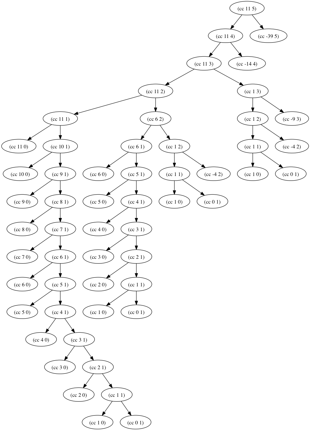The order of growth of the space is linear in relation to the amount to be changed and the number of kinds of coins. In other words, it is 𝛳(a + k), where a = amount and k = kinds of coins. Nonetheless, in our setup the kinds of coins is constant, so we are left with 𝛳(a).

The recurrent relation in regard to the number of steps is $T(a,k)=T(a,k-1) + T(a-V_k,k)$ , where $V_k$ is the monetary amount denoted by the matching type of coin. By looking at the leftmost branch of the above tree it is easy to discern, that $T(a,1)=2a+1$ (this stems from the way how the recursive logic is specified in our program). By looking at the middle of the tree we may notice, that roughly $T(a,2)={\frac a {V_2}}T(a,1)$ . Recall that the amount is decreased each time by $V_k$ when we recurse with the same number of kinds of coins. In general, $T(a,k)={\frac a {V_k}}T(a,k-1)$ . Therefore, the order of growth in the number of steps is O( $a^k$ ) (in our case k is fixed to 5). You should remember that this is a very crude approximation, and only tells us the upper bound.

Exercise 1.15

Procedure p is applied 5 times while evaluating (sine 12.15). On each call the angle is divided by 3, which means there are around ${\log_3 a}$ such divisions. This also defines the order of growth in space and number of steps of our procedure, i.e., both of them are 𝛳(log a) (the base of the logarithm doesn't matter).

Exercise 1.16

See the file chapter1/exercise1.16.rkt.

Exercise 1.17

See the file chapter1/exercise1.17.rkt.

Exercise 1.18

See the file chapter1/exercise1.18.rkt.

Exercise 1.19

See the file chapter1/exercise1.19.rkt.

Exercise 1.20

In the applicative-oder evaluation there are four calls to remainder. The output below shows the traced version of the remainder procedure while evaluating (gcd 206 40). See the file chapter1/exercise1.20.rkt how to setup such traces in DrRacket.

> (gcd 206 40)
>(remainder-traced 206 40)
<6
>(remainder-traced 40 6)
<4
>(remainder-traced 6 4)
<2
>(remainder-traced 4 2)
<0
2

In the normal-order evaluation there are 18 calls to remainder. The if special-form behaves the same way in both modes. In normal-oder regime everything is expanded first, then reduced. The predicate is evaluated in each iteration, but since parameters are replaced with expressions (instead of values as in applicative-oder mode) these gets longer and longer each time. Therefore, the predicate will contain an increasing number of remainder procedure calls.

Exercise 1.21

The smallest divisors are (in the same order as asked in the SICP book): 199, 1999, and 7. This exercise demonstrates how intuition may easily fool us in mathematics.

Exercise 1.22

The output of one test run has produced the following output (other runs have shown similar figures):

1001
1003
1005
1007
1009 *** 0.00390625
1011
1013 *** 0.0029296875
1015
1017
1019 *** 0.00390625
STOP
10001
10003
10005
10007 *** 0.010009765625
10009 *** 0.0087890625
10011
10013
10015
10017
10019
10021
10023
10025
10027
10029
10031
10033
10035
10037 *** 0.009033203125
STOP
100001
100003 *** 0.026123046875
100005
100007
100009
100011
100013
100015
100017
100019 *** 0.026123046875
100021
100023
100025
100027
100029
100031
100033
100035
100037
100039
100041
100043 *** 0.02587890625
STOP
1000001
1000003 *** 0.0791015625
1000005
1000007
1000009
1000011
1000013
1000015
1000017
1000019
1000021
1000023
1000025
1000027
1000029
1000031
1000033 *** 0.079833984375
1000035
1000037 *** 0.083984375
STOP

√10 is 3.16, so we should expect about a factor of 3 increase in execution times between each subsequent range. This rule is indeed reflected in the report (especially including the relation between ranges starting at 100,000 and 1,000,000). See the file chapter1/exercise1.22.rkt for the full solution of instrumenting the execution as well as how to implement the search-for-primes procedure (it stops the search after finding the first three primes in a range).² At any rate, the result is compatible with the notion that programs on my machine run in time proportional to the number of steps required for the computation.

Another source of variance is related to the definition of the runtime procedure. If it also counts garbage-collection time, then the output may be inaccurate. This remarks also applies to the next two exercises.

Exercise 1.23

Here is the output from a typical run:

1001
1003
1005
1007
1009 *** 0.004150390625
1011
1013 *** 0.004150390625
1015
1017
1019 *** 0.003173828125
STOP
10001
10003
10005
10007 *** 0.008056640625
10009 *** 0.008056640625
10011
10013
10015
10017
10019
10021
10023
10025
10027
10029
10031
10033
10035
10037 *** 0.007080078125
STOP
100001
100003 *** 0.01904296875
100005
100007
100009
100011
100013
100015
100017
100019 *** 0.02001953125
100021
100023
100025
100027
100029
100031
100033
100035
100037
100039
100041
100043 *** 0.01611328125
STOP
1000001
1000003 *** 0.049072265625
1000005
1000007
1000009
1000011
1000013
1000015
1000017
1000019
1000021
1000023
1000025
1000027
1000029
1000031
1000033 *** 0.0498046875
1000035
1000037 *** 0.058837890625
STOP

We may see an improvement, but clearly not a factor of 2. Moreover, for lower ranges the speedup is less significant; the measurement is susceptible to disturbances in the environment and depends upon the resolution of our timer. The new procedure next is somewhat slower than the built-in addition, so this also impact the result. However, the gain is worthwhile, and this is a good optimization of our code. See also the file chapter1/exercise1.23.rkt.

Exercise 1.24

Here is the output from a typical run:

1001
1003
1005
1007
1009 *** 0.007080078125
1011
1013 *** 0.007080078125
1015
1017
1019 *** 0.007080078125
STOP
10001
10003
10005
10007 *** 0.008056640625
10009 *** 0.0087890625
10011
10013
10015
10017
10019
10021
10023
10025
10027
10029
10031
10033
10035
10037 *** 0.0087890625
STOP
100001
100003 *** 0.009033203125
100005
100007
100009
100011
100013
100015
100017
100019 *** 0.009033203125
100021
100023
100025
100027
100029
100031
100033
100035
100037
100039
100041
100043 *** 0.009033203125
STOP
1000001
1000003 *** 0.010009765625
1000005
1000007
1000009
1000011
1000013
1000015
1000017
1000019
1000021
1000023
1000025
1000027
1000029
1000031
1000033 *** 0.010986328125
1000035
1000037 *** 0.010986328125
STOP

The average time in the 1000 range is around 0.007, and in the 1000000 one is about 0.011. In case of truly logarithmic behavior doubling the number of digits (moving from the 1000 toward the 1000000 range) should double the execution time. In our case, the growth isn't that fast. However, by increasing the ranges we may see, that the growth of the execution time is slightly faster. This may be explained with the slowdown in handling large numbers (including the routine to produce large enough random numbers). See also the file chapter1/exercise1.24.rkt.

Exercise 1.25

She isn't correct, and the reason is explained in the SICP book (see footnote 46). Working with smaller numbers improves performance.

Exercise 1.26

The expression (expmod base (/ exp 2) m) is evaluated twice in this version of the expmod procedure. So, any gain by halving the exponent is eliminated with such redundant evaluations. We would arrive to a process reflecting a tree with $2^n$ nodes of depth $\log n$ . We know that $\log {2^n}$ is simply n.

Exercise 1.27

See the file chapter1/exercise1.27.rkt.

Exercise 1.28

See the file chapter1/exercise1.28.rkt.

Exercise 1.29

See the file chapter1/exercise1.29.rkt. The program outputs the exact value of 0.25 for both inputs, which is much better than in the case of direct summation.

Exercise 1.30

See the file chapter1/exercise1.30.rkt.

Exercise 1.31

See the file chapter1/exercise1.31.rkt.

Exercise 1.32

See the file chapter1/exercise1.32.rkt.

Exercise 1.33

See the file chapter1/exercise1.33.rkt.

Exercise 1.34

The interpreter will report an error, that it cannot apply 2 to its arguments (2 isn't a procedure that expects one argument). This happens on the second call to f (inside f's body), when the interpreter hits the expression (2 2).

Exercise 1.35

See the file chapter1/exercise1.35.rkt.

Exercise 1.36

Here is the output from the two runs:

1.5 --> 17.036620761802716
17.036620761802716 --> 2.436284152826871
2.436284152826871 --> 7.7573914048784065
7.7573914048784065 --> 3.3718636013068974
3.3718636013068974 --> 5.683217478018266
5.683217478018266 --> 3.97564638093712
3.97564638093712 --> 5.004940305230897
5.004940305230897 --> 4.2893976408423535
4.2893976408423535 --> 4.743860707684508
4.743860707684508 --> 4.437003894526853
4.437003894526853 --> 4.6361416205906485
4.6361416205906485 --> 4.503444951269147
4.503444951269147 --> 4.590350549476868
4.590350549476868 --> 4.532777517802648
4.532777517802648 --> 4.570631779772813
4.570631779772813 --> 4.545618222336422
4.545618222336422 --> 4.562092653795064
4.562092653795064 --> 4.551218723744055
4.551218723744055 --> 4.558385805707352
4.558385805707352 --> 4.553657479516671
4.553657479516671 --> 4.55677495241968
4.55677495241968 --> 4.554718702465183
4.554718702465183 --> 4.556074615314888
4.556074615314888 --> 4.555180352768613
4.555180352768613 --> 4.555770074687025
4.555770074687025 --> 4.555381152108018
4.555381152108018 --> 4.555637634081652
4.555637634081652 --> 4.555468486740348
4.555468486740348 --> 4.555580035270157
4.555580035270157 --> 4.555506470667713
4.555506470667713 --> 4.555554984963888
4.555554984963888 --> 4.5555229906097905
4.5555229906097905 --> 4.555544090254035
4.555544090254035 --> 4.555530175417048
4.555530175417048 --> 4.555539351985717
END
1.5 --> 9.268310380901358
9.268310380901358 --> 6.185343522487719
6.185343522487719 --> 4.988133688461795
4.988133688461795 --> 4.643254620420954
4.643254620420954 --> 4.571101497091747
4.571101497091747 --> 4.5582061760763715
4.5582061760763715 --> 4.555990975858476
4.555990975858476 --> 4.555613236666653
4.555613236666653 --> 4.555548906156018
4.555548906156018 --> 4.555537952796512
4.555537952796512 --> 4.555536087870658
END

Apparently, the first instance has many oscillations, which prevents the program to quickly approach the final result. The second one applies the technique of average damping. With damping there are much less iterations, as the program converges quite quickly to the desired output. See also the file chapter1/exercise1.36.rkt.

Exercise 1.37

After setting k to be 11 we may get an approximation that is accurate to 4 decimal places (the value 0.6180). See also the file chapter1/exercise1.37.rkt. Observe the difference between the recursive and iterative variants. The former uses a top-down, while the latter a bottom-up accumulation of the result. A bottom-up buildup of the result is the cornerstone of the Dynamic Programming technique.

Exercise 1.38

See the file chapter1/exercise1.38.rkt.

Exercise 1.39

See the file chapter1/exercise1.39.rkt.

Exercise 1.40

See the file chapter1/exercise1.40.rkt. Notice that the procedure cubic is returning a procedure as its return value.

Exercise 1.41

See the file chapter1/exercise1.41.rkt. The expression (((double (double double)) inc) 5) evaluates to 21. To better understand this, the following two "rewrites" are equivalent to the previous expression:

(((double double) ((double double) inc)) 5)
((double (double (double (double inc)))) 5)

Unfolding the last one from right to left would result in 16 chained inc calls. This means increasing 5 by 16, which gives 21.

Exercise 1.42

See the file chapter1/exercise1.42.rkt.

Exercise 1.43

See the file chapter1/exercise1.43.rkt.

Exercise 1.44

See the file chapter1/exercise1.44.rkt. To obtain the n-fold smoothed function you should use ((repeated smooth n) f).

Exercise 1.45

See the file chapter1/exercise1.45.rkt. For experimenting with the number of times to repeat the average-damp procedure, I've implemented the test procedure (see the source code). It computes the n-root from the interval of [k, n] for number 3. With a single average-damp it blocks on the fourth root, as hinted in the SICP book. This case only proves that the test harness is properly setup. With 2 damps here is the output from the test run:

> (test 4 100)
4: 3.000000000000033
5: 3.0000008877496294
6: 2.999996785898161
7: 3.0000041735235943
8:

This time it blocks on the 8th root. Here is the try with 3 damps:

> (test 8 100)
8: 3.0000000000173292
9: 2.9999993492954617
10: 2.9999982624745742
11: 3.000002135562327
12: 3.000003243693911
13: 2.9999967990518366
14: 2.9999959148601363
15: 3.000004202219401
16:

Now it stops at the 16th root. The pattern starts to emerge, but let we try once more:

> (test 16 100)
16: 3.0
17: 2.999999781018786
18: 2.999999718211633
19: 3.0000006119674296
20: 2.9999991328797613
21: 3.0000011544632317
22: 2.9999984489401497
23: 3.000002128951781
24: 2.9999970572288652
25: 2.999997795764423
26: 3.000002754128255
27: 3.0000033809765188
28: 2.9999964726697
29: 2.9999955770185953
30: 3.000004433931018
31: 3.0000046736946313
32:

So, for k damps it will block on the $2^{k+1}$ th root. Therefore, the required number of damps is ${\lfloor {\log_2 n} \rfloor}$ . When we incorporate this into our procedure, then it smoothly runs for (test 2 100).

Exercise 1.46

See the file chapter1/exercise1.46.rkt.

¹. The diagram is auto-generated by an altered counting program, that emits GraphViz commands in the DOT language. You may get this version from here. ↩

². The procedure start-prime-test in the SICP book contains an error. Namely, the if should be changed to cond. ↩