Second Chapter

This chapter contains solutions to exercises from the second chapter of the SICP book.

I am using '() instead of nil in all solutions (I have not included the (define nil '()) fragment in the listings).

Exercise 2.1

See the file chapter2/exercise2.1.rkt. The solution uses some Racket's built-in procedures (like, gcd, sgn, etc.).

The version of the gcd from the SICP book isn't quite correct! It returns a negative common divisor if any argument is negative. Racket's gcd always properly returns a positive integer, though.

Exercise 2.2

See the file chapter2/exercise2.2.rkt.

Exercise 2.3

See the file chapter2/exercise2.3.rkt. The solution contains two versions of the rectangle: with 2 line segments, and with one line segment (stored as pair of points). You can try out each one by switching commented sections in the file. At any rate, the reusable procedures perimeter and area are defined in terms of width and height of a rectangle. These are the abstraction barriers that shield upper layers from internal representation details of a rectangle.

Exercise 2.4

The cdr procedure is defined as follows:

(define (cdr z)
  (z (lambda (p q) q)))

The pair is represented as a procedure with one parameter, which serves as an operator in the expression comprising the body of the lambda procedure. It receives two arguments (x and y), that are reflecting the values passed to cons. Both car and cdr function in a similar fashion. They call the procedure returned by cons, and pass a new procedure as argument, that returns its first or second argument (depending on whether it is car or cdr, respectively). Those arguments are exactly the bound values x and y.

Exercise 2.5

See the file chapter2/exercise2.5.rkt.

Exercise 2.6

See the file chapter2/exercise2.6.rkt.

Exercise 2.7

See the file chapter2/exercise2.7.rkt.

Exercise 2.8

See the file chapter2/exercise2.8.rkt.

Exercise 2.9

The width of an interval [a,b] is $\frac {b-a} 2$ . Let us see what happens, when we add two intervals: [a,b]+[c,d]=[a+c,b+d]. The width of the sum is given by ${\frac {(b+d)-(a+c)} 2}={\frac {(b-a)-(d-c)} 2}={\frac {b-a} 2}-{\frac {d-c} 2}$ . The last expression is basically the difference of the widths of the participating intervals. Similarly, we can shows that the width of the difference is the sum of the widths of the participating intervals.

Suppose we have two intervals [1,2] and [2,3] (having the same width $\frac 1 2$ ). If we multiply them by an interval [2,4], then we will get [1,2]*[2,4]=[2,8] and [2,3]*[2,4]=[4,12]. But these have different widths, so it cannot be the case that the product is a function of widths of the participating intervals. Since, division is defined in the terms of multiplication, the same reasoning applies, too.

Exercise 2.10

See the file chapter2/exercise2.10.rkt.

Exercise 2.11

See the file chapter2/exercise2.11.rkt. Actually, the problem is ill formulated. Namely, there are lot more cases if we differentiate whether any interval contains zero as its lower or upper bound (an extreme case of [0,0] doesn't even require a multiplication). The primitive sgn procedure does handle zero as a special case.

This exercise shows how aggressive optimization may ruin maintainability. The solution is also instructive to get an insight into the required amount of extra energy and creativity to keep readability and comprehensibility at a decent level. Such optimizations should never be done without first profiling the system to ensure you have a clear understanding where is the bottleneck.

Exercise 2.12

See the file chapter2/exercise2.12.rkt.

Exercise 2.13

Suppose we have two intervals defined with centers $c_1$ , $c_2$ and percentage tolerances $p_1$ , $p_2$ , respectively. Furthermore, the percentages are represented as numbers from the interval [0,1] (they are already divided by 100). We will use the rule for [+,+]*[+,+] due to positive numbers:

$[c_1(1-p_1),c_1(1+p_1)]*[c_2(1-p_2),c_2(1+p_2)]=[c_1c_2(1-p_1)(1-p_2),c_1c_2(1+p_1)(1+p_2)]$

We will use the fact of small percentages in the next line, where $p_1p_2 \approx 0$ :

$[c_1c_2(1-p_1-p_2-p_1p_2),c_1c_2(1+p_1+p_2+p_1p_2)]=[c_1c_2(1-(p_1+p_2)),c_1c_2(1+(p_1+p_2))]$

Observe that the percentage tolerance of the product is the sum of the individual percentages.

Exercise 2.14

See the file chapter2/exercise2.14.rkt. The code contains sample expressions, and specifies the asked intervals A and B. It also calculates the parallel resistances using both variants of the formula; you will notice a significant difference. This shows that algebraically equivalent expressions par1 and par2 don't result in the same value.

Watch the huge difference between the interval A, and the result of calculating $\frac {\frac A A} {\frac 1 A}$ . The latter should equal to A. Nonetheless, the difference is quite big. This phenomena will be important in understanding the next exercise.

Exercise 2.15

Eva Lu Ator is absolutely right, which you might have already observed in the previous exercise (par2's output was more accurate). The main reason is that each occurrence of an interval variable inside a complicated expression is taken independently, which is wrong. This leads to the issue known as the dependency problem. The outcome is an interval with a much bigger uncertainty than necessary. This may lead to large widths, thus render a useless result.

Exercise 2.16

The is nicely explained in the article about Interval Arithmetic. Here is the citation that answers the question from this exercise:

"In general, it can be shown that the exact range of values can be achieved, if each variable appears only once and if f is continuous inside the box. However, not every function can be rewritten this way."

Exercise 2.17

See the file chapter2/exercise2.17.rkt.

Exercise 2.18

See the file chapter2/exercise2.18.rkt.

Exercise 2.19

See the file chapter2/exercise2.19.rkt. The order of the list coin-values doesn't affect the answer produced by cc. The generated recursive tree will be different, but the terminal nodes will remain the same. The procedure systematically processes every subproblem, and none of them are skipped by shuffling the coin-values.

Exercise 2.20

See the file chapter2/exercise2.20.rkt. You should be careful that calling (same-parity 1 2 3 4 5 6 7) and (same-parity (list 1 2 3 4 5 6 7)) is totally different! The latter will assign the whole list to x and set y to an empty list.

Exercise 2.21

See the file chapter2/exercise2.21.rkt.

Exercise 2.22

The first iterative version appends a new element to the current answer. On the other hand, the current answer contains exactly all preceding elements of the list. Therefore, each new element comes before previous ones, so the resulting list will be in reverse order.

The second iterative version will not produce a list, since the chain will not be terminated with nil (this was also an initial value of the answer parameter at the beginning of iteration). For the test example given in the SICP book the output is ((((() . 1) . 4) . 9) . 16).

Exercise 2.23

See the file chapter2/exercise2.23.rkt.

Exercise 2.24

The result printed by the interpreter is (1 (2 (3 4))). The corresponding box-and-pointer structure is presented below.

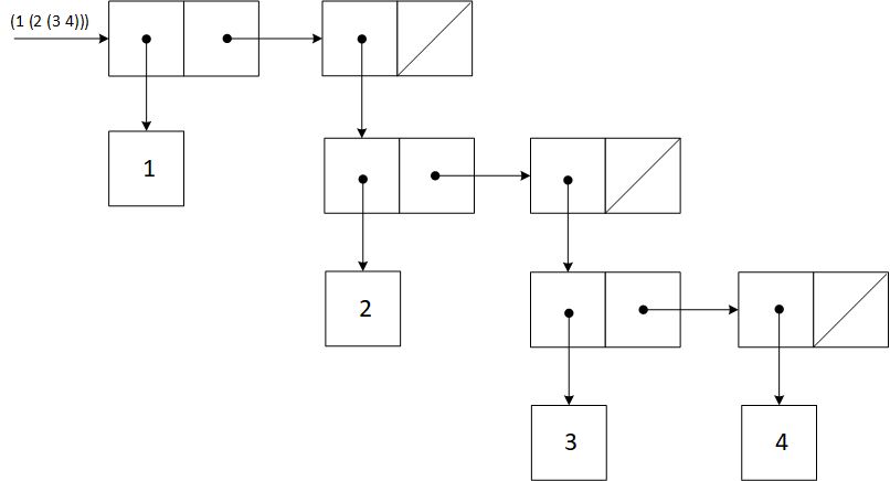
Finally, the interpretation of this as a tree is illustrated next.

Exercise 2.25

(cadr (caddr '(1 3 (5 7) 9)))
(caar '((7)))
(cadr (cadr (cadr (cadr (cadr (cadr '(1 (2 (3 (4 (5 (6 7))))))))))))

Exercise 2.26

The responses are as follows (in the same order as asked in the SICP book):

(1 2 3 4 5 6)
((1 2 3) 4 5 6)
((1 2 3) (4 5 6))

Exercise 2.27

See the file chapter2/exercise2.27.rkt.

Exercise 2.28

See the file chapter2/exercise2.28.rkt.

Exercise 2.29

See the file chapter2/exercise2.29.rkt. This contains solutions for parts a-c.

Part d

Only the right-branch and branch-structure selectors must be modified; the cadr must be replaced by cdr.

Exercise 2.30

See the file chapter2/exercise2.30.rkt.

Exercise 2.31

See the file chapter2/exercise2.31.rkt.

Exercise 2.32

See the file chapter2/exercise2.32.rkt. The solution is based upon the divide and conquer algorithm. The subsets may be generated using the following wishful thinking recursive process:

All subsets of an empty set is an empty set (exit condition, or base case).
For any non-empty set take out its first element.
Attach the first element from step 2 to all subordinate subsets.

Here, the wishful part is that we pretend we know how to generate all subsets of a smaller set (when we take out the first element from the original set).

Exercise 2.33

See the file chapter2/exercise2.33.rkt.

Exercise 2.34

See the file chapter2/exercise2.34.rkt.

Exercise 2.35

See the file chapter2/exercise2.35.rkt.

Exercise 2.36

See the file chapter2/exercise2.36.rkt.

Exercise 2.37

See the file chapter2/exercise2.37.rkt.

Exercise 2.38

The values of the expressions are (in the same order as asked in the SICP book):

3/2
1/6
(1 (2 (3 ())))
(((() 1) 2) 3)

The operator should be commutative to guarantee that fold-right and fold-left will produce the same values for any sequence.

Exercise 2.39

See the file chapter2/exercise2.39.rkt.

Exercise 2.40

See the file chapter2/exercise2.40.rkt.

Exercise 2.41

See the file chapter2/exercise2.41.rkt.

Exercise 2.42

See the file chapter2/exercise2.42.rkt. The data structure for the board was somehow suggested by the provided skeleton queens. It is possible to avoid storing rows in positions by relying on the element's index inside a list. For example, an item with index 3 would designate the column value for row 3.

Exercise 2.43

In Louis Reasoner's version (assume we are at column k) each new row redundantly solves the k-1 case. Therefore, we may establish the following recurrent relation: $T(N,k)=N*T(N,k-1)$ , where N is the board size. This entails an order of growth O( $N^N$ ). The original version had solved each subordinate problem only once. Roughly speaking Louis's version would need $8^8T$ time to solve the eight-queens puzzle (this is an astonishingly long time).

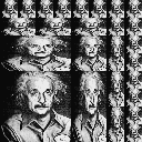
Exercise 2.44

See the file chapter2/exercise2.44.rkt. The next couple of solutions rely on the SICP Picture Language library.¹ Below is the result of executing the (paint (up-split einstein 3)) statement.

Here is the citation from the SICP book about painters:

"A painter is represented as a procedure that, given a frame as argument, draws a particular image shifted and scaled to fit the frame. That is to say, if p is a painter and f is a frame, then we produce p's image in f by calling p with f as argument."

The previously mentioned library expects a call to paint with a painter as an argument to render an image.

Exercise 2.45

See the file chapter2/exercise2.45.rkt.

Exercise 2.46

See the file chapter2/exercise2.46.rkt.

Exercise 2.47

See the file chapter2/exercise2.47.rkt.

Exercise 2.48

See the file chapter2/exercise2.48.rkt.

Exercise 2.49

See the file chapter2/exercise2.49.rkt.

Exercise 2.50

See the file chapter2/exercise2.50.rkt.

The code is altered a bit to accommodate the SICP Picture library (see the comment for exercise 2.44). The painter is commented out inside the body, as it isn't used. Nonetheless, the signatures were kept to comply with the SICP book.

Exercise 2.51

See the file chapter2/exercise2.51.rkt.

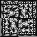
Exercise 2.52

See the files chapter2/exercise2.52a-c.rkt. Below is the output from the new corner-split painter, as suggested in the SICP book.

Finally, below is the effect of altering the square-limit procedure.

Exercise 2.53

Here is the output from the interpreter in the same order as asked in this exercise:

(a b c)
((george))
((y1 y2))
(y1 y2)
#f
#f
(red shoes blue socks)

Exercise 2.54

See the file chapter2/exercise2.54.rkt.

Exercise 2.55

The expression from the book is equivalent to (car (list 'quote 'abracadabra)), as explained in the SICP book's footnote 34. Now it is easy to see why the output is quote.

Exercise 2.56

See the file chapter2/exercise2.56.rkt.

Exercise 2.57

See the file chapter2/exercise2.57.rkt. Changing only the augend and multiplicand selectors indeed accomplishes the goal, but it is far from perfect. Here are two examples demonstrating the weirdness of the output:

(deriv '(* c x y (+ x 3)) 'x)
(* c (+ (* x y) (* y (+ x 3))))

(deriv '(* x y (+ x 3) c) 'x)
(+ (* x (* y c)) (* y (+ x 3) c))

The second result, although totally correct, is definitely less readable than the first one. Nonetheless, both expressions are algebraically equivalent.

Exercise 2.58

Part a

See the file chapter2/exercise2.58a.rkt. There are only trivial changes to predicates, selectors and constructors.

Part b

See the file chapter2/exercise2.58b.rkt. Notice the new abstraction barrier established with the following procedures: parse, first-arg, and second-arg. These provide a nice base for predicates and selectors, whose implementation is trivial.

The parsing logic leverages the ordering of rules inside the derivation engine; a similar tactic is used in the SICP book for the adjoin-term procedure, as explained there in footnote 59. Namely, the call to sum? precedes product?, which is exactly what we need to simplify the implementation. Of course, a proper way is to let precedence of rules/operators be driven by a separate module; it could provide either the precedence of rules inside the derivation engine, or the operators inside the parser. Nonetheless, whatever decision is required it is now postponable, thankfully to the newly introduced layer between predicates/selectors and the underlying representation. In a sense, the crux of this exercise is to discover the need for this shield.

Exercise 2.59

See the file chapter2/exercise2.59.rkt.

Exercise 2.60

See the file chapter2/exercise2.60.rkt. The adjoin-set is now O(1), and the union-set O(n). The other two are about the same (although the variants using duplicates would be slower depending upon the number of duplicated elements). The new version is better, when there are lots of additions of new elements (preferably unique ones to avoid repetition) with rare searches (either for an element membership or intersection). The variant with duplicates potentially eats up more memory, so isn't a good option in memory constrained devices. Again, this is only true if the level of duplication is high.

As the test case in the code shows, the intersection may also contain multiple elements. For this to be formally specified we need to augment the text of footnote 37 in the SICP book with the following statement:

For any sets S and T and any object x, (element-of-set? x (intersection-set S T)) is equal to (and (element-of-set? x S) (element-of-set? x T)) (informally: "The elements of (intersection S T) are the elements that are both in S and in T'').

Exercise 2.61

See the file chapter2/exercise2.61.rkt.

Exercise 2.62

See the file chapter2/exercise2.62.rkt.

Exercise 2.63

Part a

The two procedures produce the same result for every tree, i.e., they perform an in-order traversal of a tree. Such a traversal returns back the leafs in sorted order. For all trees in figure 2.16 the output is (1 3 5 7 9 11).

Part b

The two procedures don't have the same order of growth in the number of steps required to convert a balanced tree with n elements to a list. The tree->list-2 grows more slowly. tree->list-1 is appending sublists at each level (requiring about n/2 steps for balanced trees), which is avoided in the second variant. Thus, the first version has an order of growth O(n* log n), and the second one O(n).

Exercise 2.64

Part a

The partial-tree procedure recursively transforms the list into a balanced tree. At each stage, the procedure calculates the number of elements in the left branch, and creates it recursively. Afterward, it chooses the middle element, which is going to be the root of the current subtree. It then creates the right branch recursively, and forms a tree from these elements. Finally, it produces the required data structure containing the produced tree and the remaining elements. Of course, the latter will be empty for all stages except possibly for the first level.

Below is the fixed version of the print-tree procedure from the associated Instructor's Manual for the SICP book (the published version has a missing else branch in the space-to procedure, since it uses if instead of cond).⁴ The listing also shows a sample call for the list asked in this exercise.

(define (print-tree tree level)
  (define (space-to n)
    (cond ((not (= n 0))
           (display " ")
           (space-to (- n 1)))))
  (cond ((null? tree) 'done)
        (else (newline)
              (space-to level)
              (display (entry tree))
              (print-tree (left-branch tree) (+ level 1))
              (print-tree (right-branch tree) (+ level 1)))))

(print-tree (list->tree '(1 3 5 7 9 11)) 0)

Next is the printout of the balanced tree:

Node 1 has only a left branch with node 3, and node 9 has two branches.

Part b

The number of steps required by list->tree to convert a list of n elements is equal to $\sum\limits_{k=1}^{log_2 n} {\frac n {2^k}} \approx n$ . This gives an O(n) order of growth.

Exercise 2.65

By combining the solutions to exercises 2.62, 2.63, and 2.64 together with code from the SICP book, we can devise the following solution (it also includes a simple test case):

(define (union-set set1 set2)
  (list->tree (union-set-list (tree->list set1)
                              (tree->list set2))))

(define (intersection-set set1 set2)
  (list->tree (intersection-set-list (tree->list set1)
                                     (tree->list set2))))

(define set1 (list->tree '(1 2 3 4 5 6 7 8)))
(define set2 (list->tree '(2 4 6 8 10 12)))

(print-tree (union-set set1 set2) 0)
(print-tree (intersection-set set1 set2) 0)

The intersection-set-list and union-set-list are the intersection-set and union-set procedures, that work with ordered lists. Moreover, the tree->list procedure is the second variant from exercise 2.63. Since all these auxiliary procedures are O(n), and are called a constant number of times, then the resulting procedures for union-set and intersection-set are also O(n). Here is the output from running the above test case:

Exercise 2.66

(define (lookup given-key set-of-records)
  (if (null? set-of-records)
      false
      (let ((curr-record-key (key (entry set-of-records))))
        (cond ((= given-key curr-record-key)
               (entry set-of-records))
              ((< given-key curr-record-key)
               (lookup given-key (left-branch set-of-records)))
              (else (lookup given-key (right-branch set-of-records)))))))

Exercise 2.67

You need to call (decode sample-message sample-tree) to get back the message, which is (A D A B B C A).

Exercise 2.68

See the file chapter2/exercise2.68.rkt, and exercise 2.72.

Exercise 2.69

See the file chapter2/exercise2.69.rkt.

Exercise 2.70

Here is the setup code to produce the required answers:

(define lyrics-tree
  (generate-huffman-tree '((a 2) (na 16) (boom 1) (Sha 3) (Get 2) (yip 9) (job 2) (Wah 1))))
(define rock-song '(Get a job Sha na na na na na na na na Get a job Sha na na na na na na na na Wah yip yip yip yip yip yip yip yip yip Sha boom))
(define encoded-rock-song (encode rock-song lyrics-tree))
(length encoded-rock-song)
(* 3 (length rock-song))

84 bits are required for the Huffman, and minimum 108 for a fixed-length code encoding.

Exercise 2.71

Observe that $\sum \limits_{i=0}^n 2^i<2^{n+1}$ for any nonnegative integer n. This gives a specific shape to the Huffman tree. Namely, each new symbol will appear on the right branch compared to the previously generated tree. The initial tree is created by symbols whose relative frequencies are 1 and 2 (the ordering does not matter). For example, below is the case with n=5:

                      {a b c d e} 31
                     /           \
                 {a b c d} 15     e 16
                 /       \
             {a b c} 7    d 8
             /     \
          {a b} 3   c 4
         /    \
      a 1      b 2

Next is the case for n=10 (you can notice the same pattern):

                                {a b c d e f g h i j} 1023
                               /                      \
                              {a b c d e f g h i} 511  j 512
                             /                    \
                            {a b c d e f g h} 255  i 256
                           /                  \
                          {a b c d e f g} 127  h 128
                         /               \    
                        {a b c d e f} 63  g 64                                         
                       /             \                                                    
                      {a b c d e} 31  f 32 
                     /           \
                 {a b c d} 15     e 16
                 /       \
             {a b c} 7    d 8
             /     \
          {a b} 3   c 4
         /    \
      a 1      b 2

Only one bit is required to encode the most frequent symbol. The least frequent symbol demands n-1 bits.

Exercise 2.72

The number of steps needed to encode the most frequent and least frequent symbols in the alphabet (using the implementation of exercise 2.68) are O(n) and O( $n^2$ ), respectively. Of course, if the encoding routine is altered to first look into the right branch, then the best case would be O(1)!

Exercise 2.73

Part a

Looking at the figure 2.22 from the SICP book, the system has introduced a polymorphic deriv operation, which is implemented differently by modules handling summation and multiplication (very similar how generic operations real-part, imag-part, magnitude and angle were done for complex numbers). Thankfully to the data-directed programming approach there is no need to modify the generic deriv procedure each time a new rule is added to the system (like the exponentiation rule).

The predicates number? and variable? work at a lower abstraction layer.² Moreover, their behavior is independent of the type of the operator inside an expression.

Part b

See the file chapter2/exercise2.73.rkt. The ch2support.scm file was not used, as it is obsolete (instead Racket's built-in hash table was leveraged).

Part c

This is bundled inside the same file chapter2/exercise2.73.rkt to avoid repeating the boilerplate code.

Part d

We would only need to correspondingly switch inside each package the order of arguments in the put statement for installing the operator specific deriv procedure.

Exercise 2.74

See the file chapter2/exercise2.74.rkt. This contains answers to parts a-c.

Part a

The division file must be tagged with a division identifier (in our case it is division1). Also, the records must have an employee name as their primary key.

Part b

The record returned from the get-record procedure must be properly tagged with a division identifier. This is required for get-salary to be able to call the division specific salary selector.

Part c

The method to find an employee relies on the generic get-record procedure, so it will work with all sorts of division files.

Part d

A new company should install the appropriate package using the provided sample as a starting point. Note the stuff commented as "interface to the rest of the system."

Exercise 2.75

(define (make-from-mag-ang r a)
  (define (dispatch op)
    (cond ((eq? op 'real-part) (* r (cos a)))
          ((eq? op 'imag-part) (* r (sin a)))
          ((eq? op 'magnitude) r)
          ((eq? op 'angle) a)
          (else (error "Unknown op -- MAKE-FROM-MAG-ANG" op))))
  dispatch)

Exercise 2.76

Each approach has benefits and drawbacks as enrolled below:

Generic operations with explicit dispatch: this is straightforward to implement and understand. Everything is explicit in the code, and debugging is fully supported by an IDE. The downside is that adding a new data type requires touching existing code (especially cumbersome with many generic operations). This is best exemplified in the exercise 2.56.
Data-directed style: this option would be most appropriate for a system in which new operations must often be added.
Message-passing style: this choice would be most appropriate for a system in which new data types must often be added.

Any complex system will, during its evolution, undergo expansions in both directions: data types and operations. Therefore, it isn't easy to make a unanimous decision. We can also see this problem in modern programming languages, which usually support multitude of paradigms (the most popular combination is the mixture of object-orientation with functional programming style).

I suggest you to also read the discussion in the Instructor's Manual for the SICP book (see section 2.4.3) regarding the maintenance of a dispatch table in case some data type specific operation is modified.

Exercise 2.77

Here we have a two-level tag system. The details of tracing through all the procedures called in evaluating the expression (magnitude z), where z is the object shown in figure 2.24 of the SICP book, are enrolled below:

The generic magnitude procedure is invoked first with z, which relies on apply-generic to forward the request to the type specific variant.
The apply-generic calls the same generic magnitude procedure again, this time stripping of the outer complex tag. Observe, that the complex variant was just a redirection toward the same generic operation.
The second time magnitude calls via apply-generic the rectangular or polar version of the magnitude procedure.

Exercise 2.78

See the file chapter2/exercise2.78.rkt.

In the subsequent solutions there are lots of boilerplate code, which are repeated for the sake of completeness. The aim is to keep each solution self-contained for better clarity. Moreover, each solution builds upon the previous one (in most cases).

Exercise 2.79

See the file chapter2/exercise2.79.rkt. Notice that equ? for a Scheme number is simply =.

Exercise 2.80

See the file chapter2/exercise2.80.rkt. Notice that =zero? for a Scheme number is simply zero?.

Exercise 2.81

Part a

If we call exp with two complex numbers as arguments the apply-generic procedure will enter an infinite loop.

Part b

Coercion with arguments of the same type must be prevented in apply-generic to avoid an endless loop.

Part c

See the file chapter2/exercise2.81.rkt.

Exercise 2.82

See the file chapter2/exercise2.82.rkt. Below is the important citation from the SICP book (that may be easily generalized to multiple arguments), that answers the question about limitations of the proposed approach:

"On the other hand, there may be applications for which our coercion scheme is not general enough. Even when neither of the objects to be combined can be converted to the type of the other it may still be possible to perform the operation by converting both objects to a third type."

Exercise 2.83

See the file chapter2/exercise2.83.rkt. Look into the code base to see how real numbers are represented. These are simulated via Scheme numbers using the inexact representation. The type-level procedure outputs a code for each type in the tower, which will be handy for later exercises.

Exercise 2.84

See the file chapter2/exercise2.84.rkt.

Exercise 2.85

See the file chapter2/exercise2.85.rkt. Observe that dropping should be tried only for a subset of operations. If operations are not filtered, then you will most probably enter an infinite loop.

Exercise 2.86

See the file chapter2/exercise2.86.rkt. This exercise requires a high attention to details, due to many places where the code must be tweaked. The text in the SICP book just hinted on such a possibility, though.

Exercise 2.87

See the file chapter2/exercise2.87.rkt. A polynomial is zero when all of its coefficients are zero. To integrate the polynomial package with the rest of the system, we also need dummy type specific project and raise procedures.

Exercise 2.88

See the file chapter2/exercise2.88.rkt.

Exercise 2.89

See the file chapter2/exercise2.89.rkt. Observe the need for padding the term list with zeros, if there is a gap between terms.

Exercise 2.90

See the file chapter2/exercise2.90.rkt. Although a major rework, the changes are localized only to the family of polynomial packages (there are two new ones to handle the dense and sparse representations). The only deliberate choice was to choose sparse as a default when creating an empty term list. This entails a sparse outcome if a dense and sparse polynomials are added, subtracted, or multiplied. You should look up the tests to see how all this executes.

Exercise 2.91

See the file chapter2/exercise2.91.rkt.

Exercise 2.92

See the file chapter2/exercise2.92.rkt. The ordering of variables is based on lexicographical ordering. The algorithm for converting a polynomial of P(y,x) into P(x,y) is as follows (after finding the principal variable of the two polynomials):

If the polynomial's variable is equal to the principal variable, then just return this polynomial.
Enumerate over terms of the polynomial.
For each term generate a temporary polynomial using the transformation below.
Add up all temporary polynomials to produce the converted polynomial (this is a simple application of the accumulate procedure).

$y^k(a_nx^n+a_{n-1}x^{n-1}+...+a_1x+a_0) \mapsto x^n(a_ny^k)+x^{n-1}(a_{n-1}y^k)+...+x(a_1y^k)+a_0y^k$

So, the generated polynomial is in variable x of the same order as was the term; the terms are polynomials in y of order k.

Besides the above algorithm, the code also introduces a way to raise complex numbers to polynomials. This is achieved by using a special universal variable. This is the highest ordered variable, so that the lowest term of some P(x) could be combined with the lowest term of this P(universal).

The final output may not always look as simple as it could be. Therefore, more work is required to reduce the result to a form we are accustomed to. Nonetheless, this is out of scope for this exercise.

Exercise 2.93

See the file chapter2/exercise2.93.rkt. Besides the actions told in the SICP book, the code was augmented as enrolled below:

The raise and project procedures in the rational package were altered, as rational functions are not anymore ordinary rational numbers.
The equ? procedure for polynomials was implemented to support this extension.

Exercise 2.94

See the file chapter2/exercise2.94.rkt.

Exercise 2.95

Here is the log from tracing the gcd-terms procedure:³

>(gcd-terms
  (sparse (4 11) (3 -22) (2 18) (1 -14) (0 7))
  (sparse (3 13) (2 -21) (1 3) (0 5)))
>(gcd-terms
  (sparse (3 13) (2 -21) (1 3) (0 5))
  (sparse (2 1458/169) (1 -2916/169) (0 1458/169)))
>(gcd-terms (sparse (2 1458/169) (1 -2916/169) (0 1458/169)) (sparse))
<(sparse (2 1458/169) (1 -2916/169) (0 1458/169))

The GCD (as printed in the console) is (polynomial x sparse (2 $8\frac {106} {169}$ )(1 - $17\frac {43} {169}$ ) (0 $8\frac {106} {169}$ )). If you start dividing the first terms of Q1 and Q2, then you will already get a term x $\frac {11} {13}$ . This issue is afterward propagated until completion of GCD.

Exercise 2.96

Part a

See the file chapter2/exercise2.96a.rkt.

Part b

See the file chapter2/exercise2.96b.rkt. Now we get back the P1 as GCD (see exercise 2.95).

Exercise 2.97

Part a

See the file chapter2/exercise2.97a.rkt.

Part b

See the file chapter2/exercise2.97b.rkt.

¹. See also the SICP Collections site. ↩

². At one point, there will be a need to access the primitive procedures number? or eq?, which would be impossible, if they are assimilated into the data-directed dispatch. ↩

³. DrRacket comes with a powerful tracing library, that can be turned on for some procedure by issuing (trace <procedure name>). The source code of the solution contains the command to import this library (it is commented out at the beginning of the file). ↩

⁴. DrRacket reports an error if the alternative path is missing. ↩