Third Chapter

This chapter contains solutions to exercises from the third chapter of the SICP book.

Starting from exercise 3.17, I am using Racket's mpairs, so every solution working with mutable data structures imports the scheme/mpair) package. Also, code samples use the racket/stream package. The semantics is preserved with MIT Scheme, but the names are different (for example, stream-car is stream-first).

Exercise 3.1

See the file chapter3/exercise3.1.rkt.

Exercise 3.2

See the file chapter3/exercise3.2.rkt. There is one huge limitation of the approach described in the SICP book. Namely, the input parameter to the monitored procedure cannot capture the built-in commands (like, how-many-calls? and reset-count). One way is to introduce a special invoke command with one argument, which would perform the actual call and pass the provided argument to the monitored procedure. Of course, the example in the SICP book uses a function whose parameter is a number, so this problem does not occur.

Exercise 3.3

See the file chapter3/exercise3.3.rkt. We are throwing an error for an incorrect password. See section 3.1.1 in the Instructor's Manual for SICP for a comment, what should be done if you simply want to return a message. See also the next exercise as a demonstration of this technique.

Exercise 3.4

See the file chapter3/exercise3.4.rkt. The solution contains an extra feature of warning how many failed attempts are left. Notice the usage of the inner lambda function, which is needed to "consume" the amount argument in the outer call.

Exercise 3.5

See the file chapter3/exercise3.5.rkt.

Exercise 3.6

See the file chapter3/exercise3.6.rkt.

Exercise 3.7

See the file chapter3/exercise3.7.rkt.

Exercise 3.8

See the file chapter3/exercise3.8.rkt.

We have demonstrated the code assuming that DrRacket will use left to right evaluation order for parameters. There is no such guarantee in Scheme. Therefore, it is considered a bad style to rely on such assumption.

Exercise 3.9

At first glance, as hinted in footnote 14 of the SICP book, the iterative version seems to require 2 environments more than the recursive version. The environment structure doesn't tell anything about the tail-recursive implementation of the interpreter. The recursive version requires O(n) space to keep track of deferred operations. The iterative version only needs the current frame, the other may be garbage-collected. Nonetheless, these details are not presented here.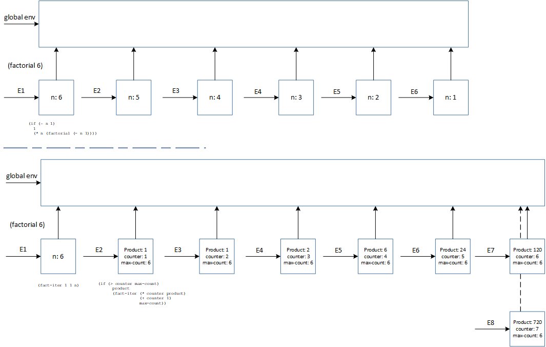

Exercise 3.10

The situation here is only different in regard to figure 3.10 from the SICP book, that that the initial-amount exists inside a "wrapper" environment E1. This is the parent environment referred by the internal lambda procedure inside the body of make-withdraw. More precisely, the let construct introduces another environment E2 (not explicitly labeled), which references E1. At any rate, the initial-amount is used only once to initialize the balance. Afterward, it just lingers there for no use. Here is the environment structure with W1 defined. The W2 would be a clone of W1, with the code pointer pointing to the shared code base with W1. The (W1 50) executes on W1's balance as depicted in figure 3.8 in the SICP book.

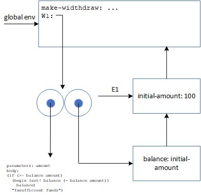
This exercise highlights one important issue with environments and lambda functions. You must be vigilant to keep environments lean and tidy. The definition of W2 will have its own initial-amount instance, despite the fact that it is same as for W1! All in all, the original version of make-withdraw is more economical.

Exercise 3.11

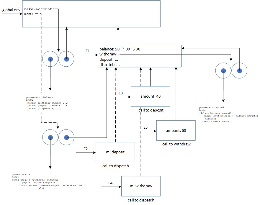
The diagram is a bit optimized with changes of the account's balance shown inside the same environment (see the arrows connecting different values). The local state of acc is kept in E1. acc2 would be a clone of acc having its own dedicated environment holding the balance and inner procedures. They would share the same code base and the global environment.

Exercise 3.12

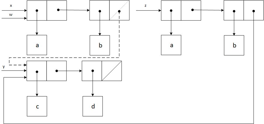
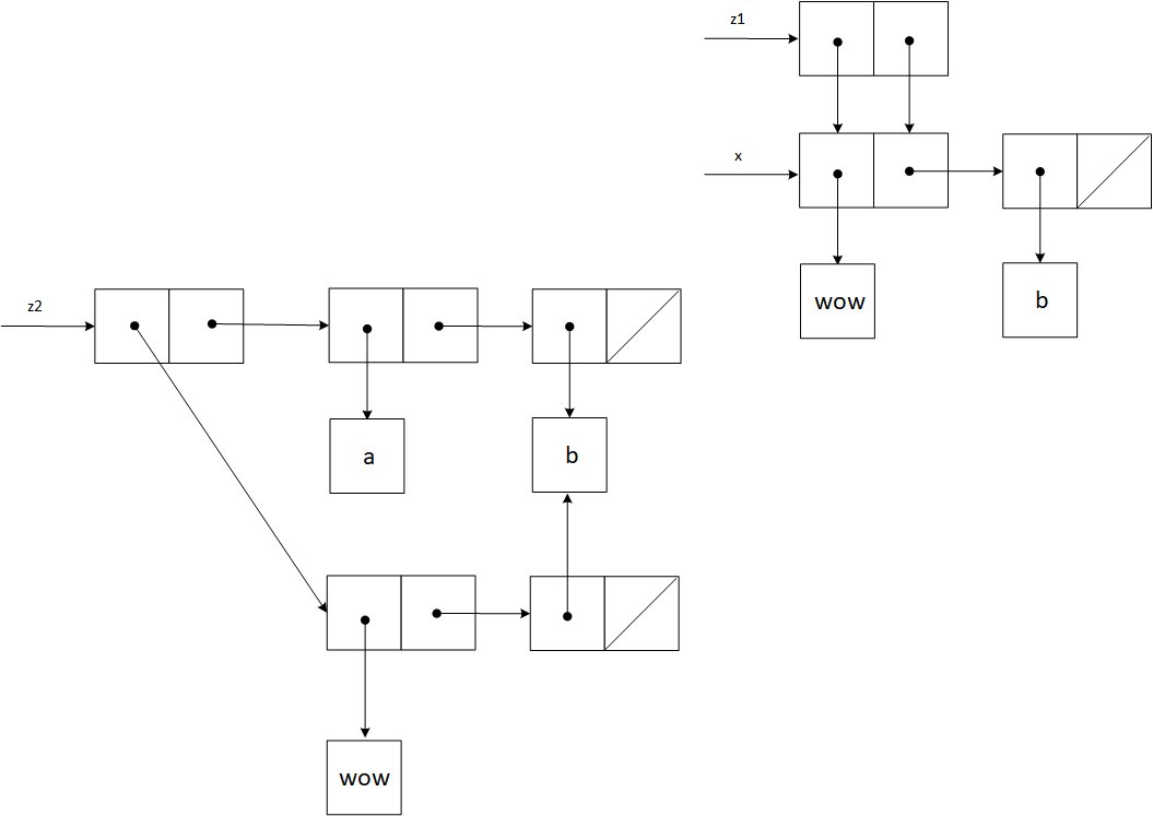
The next diagram combines the two scenarios (see the dashed elements). The first (cdr x) response will be (b), and the second one (b c d).

Exercise 3.13

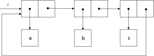
Below is the box-and-pointer diagram for z. If we try to compute (last-pair z), then the program will enter an infinite loop.

Exercise 3.14

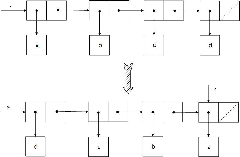
The procedure mystery inverts in-place the elements of a list. At the end, w will be (d c b a) and v will be (a), as represented below.

Exercise 3.15

Exercise 3.16

Exercise 3.17

See the file chapter3/exercise3.17.rkt. Observe the usage of memq in searching for visited pairs (the same technique is used in the next exercise.). Internally it uses eq?, which compares references. Using equal? would be wrong here, since we want to referentially compare whether we have seen some pair before, rather than looking at the content.

Exercise 3.18

See the file chapter3/exercise3.18.rkt.

Exercise 3.19

See the file chapter3/exercise3.19.rkt. ; The solution is based on the tortoise and the hare algorithm. It uses O(1) space with 2 pointers: tortoise (moves one item at a time) and hare (moves 2 items at a time). If they meet then we have a cycle. Otherwise, the hare will reach the end of the list.

For simplicity reasons, the internal variables to keep the position of tortoise and hare are introduced with define. This is not a suggested practice. It is better to use let, and define all internal procedure inside the body of let.

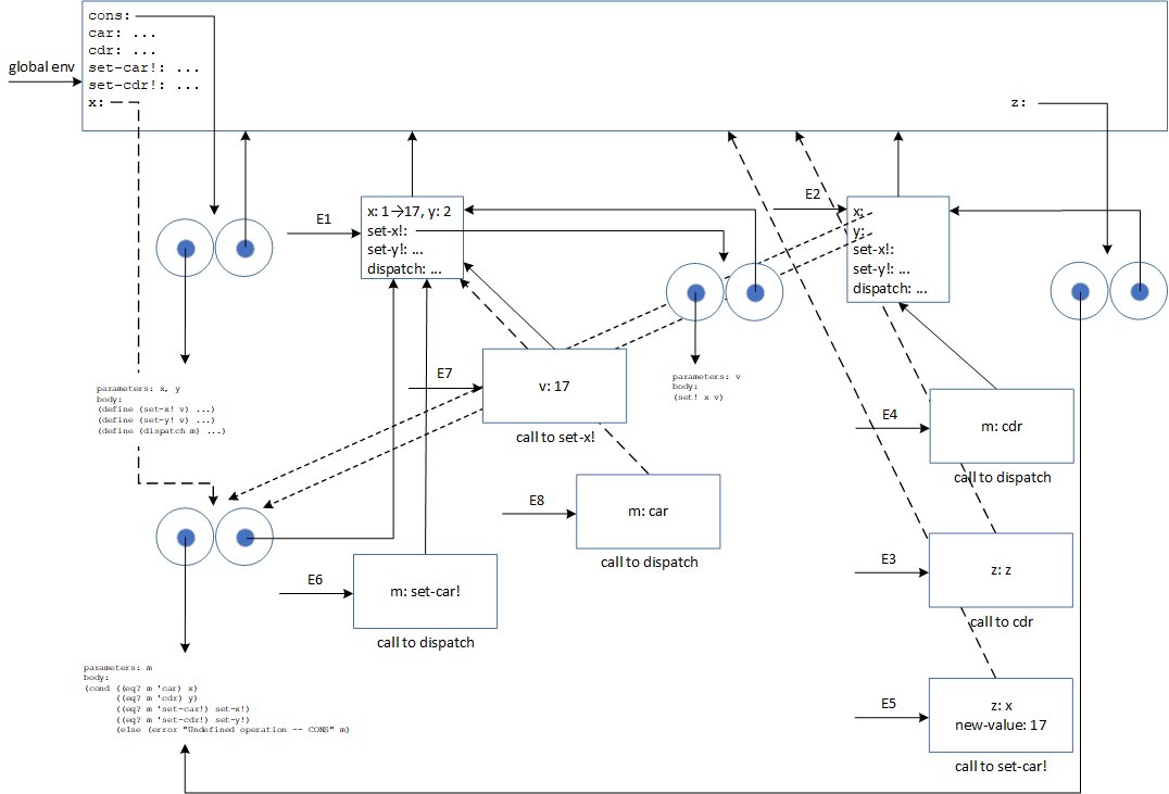
Exercise 3.20

This is quite a complex diagram. You just need to follow the ordering of environments to understand what is going on. Also, watch out where each environment points back. For example, the parent of environment E3 is the global environment (due to the static binding approach). The first element of x is altered by set-x! in environment E7. In environment E5, I've marked z: x to avoid an extra arrow on the diagram (that arrow would actually point to x).

Exercise 3.21

The front pointer is pointing at the beginning of the queue's content (list). The rear pointer is just introduced to speed up the append actions. The standard printing facility shows the content of the lists pointed at by both the front and rear pointers. This is the reason why the printout is wrong. Therefore, we just need to print the content pointed at by the front pointer. See the next exercise's solution that includes this printing procedure.

Exercise 3.22

See the file chapter3/exercise3.22.rkt.

Exercise 3.23

See the file chapter3/exercise3.23.rkt. I've used a double linked list; another possibility is to use a circular list. The latter requires careful handling of cycles.

Exercise 3.24

See the file chapter3/exercise3.24.rkt.

Exercise 3.25

See the file chapter3/exercise3.25.rkt. ; We are continuing to modify the solution of exercise 3.24. This exercise is not easy if you want to make a solution flexible, supporting many edge cases (see the test cases for some illustrations with additional comments). Also, we are making a decision here that '() denotes an empty value. Finally, non-existent composite keys are returned as false.

The specification is quite vague, and many details are left open. For example, the provided solution does not support partial matches.

Exercise 3.26

The idea is to introduce separate binary trees for each key space (in the same manner as there was a separate backbone for each key dimension in an unordered list table representation). The key spaces would be linked together via a backbone list. The lookup and insert routines would perform similarly as in exercise 3.25 (via recursive processing of a tree one key space at a time). All the procedures for working with a binary tree are presented in chapter 2. Moreover, each key space could be searched via the solution for exercise 2.66.

Exercise 3.27

The memoization assures that any particular argument n is computed only once. In the original algorithm, for some m < n, Fib(m) was generally computed multiple times. As there are n different Fibonacci numbers in a computation of Fib(n), and each of them are computed only once, the overall number of steps is O(n).

Defining memo-fib to be (memoize fib) will not help, since the original algorithm has recursive calls, and these will not hit the memoized version of fib.

Instead of environment diagrams, it is better to trace the execution of (fib 5) and (memo-fib 5) using DrRacket's tracing library. Below are the two traces. Notice, the needless computations in the original fib procedure.

; Trace of (fib 5)
>(fib 5)
> (fib 4)
> >(fib 3)
> > (fib 2)
> > >(fib 1)
< < <1
> > >(fib 0)
< < <0
< < 1
> > (fib 1)
< < 1
< <2
> >(fib 2)
> > (fib 1)
< < 1
> > (fib 0)
< < 0
< <1
< 3
> (fib 3)
> >(fib 2)
> > (fib 1)
< < 1
> > (fib 0)
< < 0
< <1
> >(fib 1)
< <1
< 2
<5
5

; Trace of (memo-fib 5)
>(memo-fib 5)
> (memo-fib 4)
> >(memo-fib 3)
> > (memo-fib 2)
> > >(memo-fib 1)
< < <1
> > >(memo-fib 0)
< < <0
< < 1
> > (memo-fib 1)
< < 1
< <2
> >(memo-fib 2)
< <1
< 3
> (memo-fib 3)
< 2
<5
5
>

Exercise 3.28

See the file chapter3/exercise3.28.rkt.

Exercise 3.29

See the file chapter3/exercise3.29.rkt. We used De Morgan's laws to express the logical or operation in terms of negation and logical and. The delay time of the or-gate is and-gate-delay + 2 * inverter-delay. The assumption is that the inverters on wires a1 and a2 may be triggered in parallel.

Exercise 3.30

See the file chapter3/exercise3.30.rkt. The total delay of the ripple-carry adder is n times the full-adder-delay. The full-adder-delay is 2 * half-adder-delay + or-gate-delay. Finally, the half-adder-delay is max(and-gate-delay + inverter-delay, or-gate-delay) + and-gate-delay.

Exercise 3.31

Without such an initialization, actions associated with wires having zero as their signal would not be executed. This could lead to wrong answers, as only part of a circuitry will "run" (those affected by change of a signal on a wire). Nonetheless, even this active circuit would run inside an improperly configured environment.

The best example is a trivial circuit with a single inverter. If you would run a simulation without an initialization, then the output wire will show zero, which is definitely wrong (a wire's default value is zero). Moreover, having an initialization is handy when putting a probe on a wire. It immediatelly displays the current signal on a wire.

Exercise 3.32

The FIFO ordering is crucial to maintain correctness. Let us analyze the and-gate as suggested in the exercise. We see that both inputs are associated with the same action. This action calculates the new value of an output signal, and schedules an update after some delay. It is important to remember, that the new value is calculated at the moment when the signal was changed, i.e., before an update.

Let us name the input wires as A and B. If the signal changes in the order of A->1 and B->0 (from A=0 and B=1), then the new values calculated by the actions associated with these wires are Output=1 for A->1 (because at this time B is still 1) and Output=0 for B->0. Since these outputs differ, they cannot be swapped. Obviously, the final output must be zero, i.e., reflect the last stable state of inputs.

Exercise 3.33

See the file chapter3/exercise3.33.rkt.

Exercise 3.34

The main flaw in Louis Reasoner's idea is that it doesn't take into account the bi-directional nature of a constraint system. In the case of the squarer constraint the only possible direction is from a to b. By setting only b the system is not capable of deciphering the value of a, i.e., it can't figure out that a is $\sqrt b$ .

Exercise 3.35

See the file chapter3/exercise3.35.rkt.

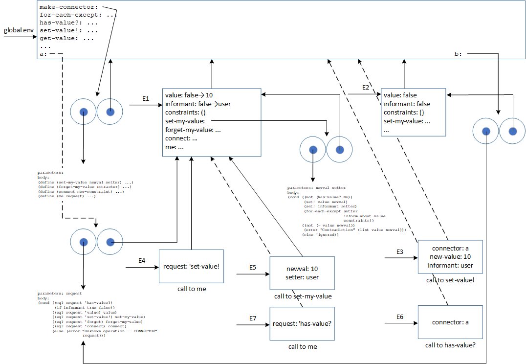
Exercise 3.36

This is again quite a complex diagram. You just need to follow the ordering of environments to understand what is going on. Also, watch out where each environment points back.

Exercise 3.37

See the file chapter3/exercise3.37.rkt.

Exercise 3.38

Part a

There are 3! possible sequential orders; balance will receive its final value from the set {50, 45, 40, 35}. Here are the possibilities:

Peter, Paul, Mary = $45
Peter, Mary, Paul = $35
Paul, Peter, Mary = $45
Paul, Mary, Peter = $50
Mary, Peter, Paul = $40
Mary, Paul, Peter = $40

Part b

Suppose all of them read out the initial balance of $100. Afterward they perform the updates in various orders (see the list above). For each of these the outcome is as follows:

Peter, Paul, Mary = $50
Peter, Mary, Paul = $80
Paul, Peter, Mary = $50
Paul, Mary, Peter = $90
Mary, Peter, Paul = $80
Mary, Paul, Peter = $90

In all of these cases the preservation of money is broken.

The list above presumes that Mary's composite action will not be interleaved after reading out the initial balance. Nonetheless, this is not true. Since she is reading the balance twice further combinations are possible. For example, Mary1, Peter, Paul, Mary2 will result in $55. Of course, all the correct answers are possible, too. This is a proof why testing concurrent programs is radically different than testing their sequential counterparts.

Exercise 3.39

Four out of five possibilities remain with the new approach. The third case (110) is prevented to happen. P1 will always read out the same value of x both times.

Exercise 3.40

The following possibilities exist with an unserialized execution (let denote the two procedures P1 and P2, respectively):

1.000.000 - (P1 full, P2 full) or (P2 full, P1 full)
100.000 - P2 reads first x, P1 full, P2 rest
10.000 - (P2 reads first and second x-es, P1 full, P2 rest) or (P1 reads first x, P2 full, P1 rest)
1.000 - P2 reads all x-es, P1 full, P2 rest
100 - P1 reads all x-es, P2 full, P1 rest

The serialized version always produces 1.000.000 = $(10^3)^2=(10^2)^3$ .

Exercise 3.41

Ben's concern is actually valid. Writing into the balance variable, may be interleaved with a read operation. It could result in a garbage (especially if balance is a "long" data type). Another issue is visibility of the latest write. These are low level technical details, and it is better to be on the safe side, and use serialized access even for reads.

Exercise 3.42

This is a good improvement in the code. The following citation from the SICP book gives an answer, why this is safe to do: "All calls to a given serializer return serialized procedures in the same set."

Exercise 3.43

We have 3 scenarios (all start out with A1=$10, A2=$20, and A3=$30), as explained next.

All accesses are sequential in some order.

At any given moment in time, only one process may perform a transaction, since a single process allocates two different accounts. At the end of each transaction, the balances will be switched by a difference. For example, A1=$10 and A3=$30 -> A1=$10-(-$20)=$30 and A3=$30+(-$20)=$10.

Each account is serialized.

Here, 2 transactions may happen in parallel. An example of this is given in the SICP book itself. Suppose that Peter has started the transaction P1 on A1 and A2. At the same time Paul has initiated an exchange P2 between A1 and A3. P1 calculates the difference to be -$10. However, before updating the accounts P2 executes fully. P2 swicthes the balances, so A1=$30 and A3=$10. Now, P1 updates these balances with the original difference of -$10. The end result is A1=$40, A2=$10 and A3=$10. Nevertheless, the total sum is still $40+$10+$10=$10+$20+$30. The reason for preserving the total sum is that each pair of accounts is always updated symmetrically with the same difference (whatever it happens to be). There is no explicit set operation with a calculated value, which would result in a totally different outcome (see the next case).

Accounts are accessed without any synchronization.

In this case all sorts of things may happen. Updates to accounts are not guaranteed to be atomic and symmetrical. Here is one scenario, where the money isn't preserved. Assume that P1 and P2 starts a transaction over different pairs of accounts. These 2 transactions will run in parallel.

P1's operations on A1 and A3	P2's operations on A2 and A3
get balance A1 ($10)	get balances A2 ($20) and A3 ($30)
get balance A3 ($30)	calculate difference (-$10)
calculate difference (-$20)	withdraw A2: read balance ($20)
withdraw A1: full ($30)	withdraw A2: calculate & set balance ($30)
deposit A3: call	deposit A3: call
deposit A3: get balance ($30)	deposit A3: get balance ($30)
deposit A3: calculate & set balance ($10)	deposit A3: calculate balance ($20)
Done	deposit A3: set balance ($20)
Done	Done

At the end, we have A1=$30, A2=$30, and A3=$20. The total sum is $80 instead of $60!

Exercise 3.44

Ben is right. The essential difference between the transfer problem and the exchange problem is about the goal. The former just wants to ensure, that the same amount is withdrawn and deposited from/into the accounts. The latter must ensure the difference is valid throughout the transaction, and that the accounts will end up swapped. This is a more brittle scenario, which does not tolerate other transactions running in parallel over the participating accounts.

Exercise 3.45

Louis version would run into a deadlock when serialized-exchange is called. Namely, the exchange procedure will acquire locks on both accounts, so neither withdraw nor deposit could later execute. The serializer described in the SICP book is not re-entrant.

Exercise 3.46

Actually this is quite easy to understand. Assume that 2 processes P1 and P2 execute at the same time the test-and-set! procedure. They both discover that the mutex is free (the cell is false), and get access to the protected section.

Exercise 3.47

Part a

The semaphore is also a shared resource, so must be protected against concurrent access. The code below introduces two helper internal procedures lock and unlock. These will shield us from the underlying implementation (mutex or test-and-set!).

(define (make-mutex-semaphore n)
  (let ((mutex (make-mutex))
        (count 0))
    (define (lock) (mutex 'acquire))
    (define (unlock) (mutex 'release))
    (define (acquire)
      (lock)
      (cond ((= count n)
             ; This is the same "busy-wait" approach as in the SICP book.
             (unlock)
             (acquire))
            (else (set! count (+ count 1))
                  (unlock))))
    (define (release)
      (lock)
      ; We must protect against over-release!
      (if (> count 0)
          (set! count (- count 1))
          'ignore)
      (unlock))
    (define (dispatch m)
      (cond ((eq? m 'acquire) (acquire))
            ((eq? m 'release) (release))
            (else (error "Unknown request -- MAKE-MUTEX-SEMAPHORE"
                         m))))
    (if (<= n 0)
        (error "Counter must be a positive integer -- MAKE-MUTEX-SEMAPHORE" n)
        dispatch)))

Part b

Only the beginning of the code is shown (that differs from the version above).

(define (make-cell-semaphore n)
  (let ((cell (mlist false))
        (count 0))
    (define (lock)
      (if (test-and-set! cell)
          (lock) ; busy-wait
          'grant-access))
    (define (unlock) (clear! cell))
...

Exercise 3.48

When processes acquire locks in order, then a deadlock cannot happen. Suppose that process P1 holds the first k locks, and needs the next lock k+1. It cannot be the case, that there is a process P2 holding the lock k+1, while waiting for some lock j<=k. P2 can only acquire the lock k+1 if it already possesses the lock j<k+1.

(define (make-account balance id)
  (define (withdraw amount)
    (if (>= balance amount)
        (begin (set! balance (- balance amount))
               balance)
        "Insufficient funds"))
  (define (deposit amount)
    (set! balance (+ balance amount))
    balance)
  (let ((protected (make-serializer)))
    (define (dispatch m)
      (cond ((eq? m 'withdraw) (protected withdraw))
            ((eq? m 'deposit) (protected deposit))
            ((eq? m 'balance) balance)
            ((eq? m 'identifier) id)
            (else (error "Unknown request -- MAKE-ACCOUNT"
                         m))))
    dispatch))

(define (serialized-exchange account1 account2)
  (let ((serializer1 (account1 'serializer))
        (id1 (account1 'identifier))
        (serializer2 (account2 'serializer))
        (id2 (account2 'identifier)))
    (let ((safe-exchange
           (if (< id1 id2)
               (serializer1 (serializer2 exchange))
               (serializer2 (serializer1 exchange)))))
      (safe-exchange account1 account2))))

It is the responsibility of a client to provide unique account identifiers.

Exercise 3.49

If ordering cannot be enforced over all resources participating in a transaction, then locks will be acquired in some arbitrary order. Suppose that we have two processes trying to lock their known batch of resources, using the proposed deadlock-avoidance technique. Furthermore, presume both of them additionally receive a new set of resources of different types {R1, R2}. None of them knows in what order to access them. If they choose different ordering, then we would stumble into the same conundrum as in the exchange problem.

Another possibility is, if the two processes receive some new resources, that are already locked by the other party. If the two processes do not exchange information about what locks they hold, then they cannot avoid a deadlock.

Exercise 3.50

See the file chapter3/exercise3.50.rkt. See the comment about this exercise in the Instructor's Manual for the SICP book. The current solution assumes that all provided streams are of the same length. Otherwise, you would need to test for the base case in the following manner (to stop if any stream runs out of elements):

(not (stream-empty? (stream-filter stream-empty? argstreams)))

Exercise 3.51

Here is the output from DrRacket (including the newlines):

55

77

In MIT/Scheme the behavior of the program would be different. It would first print 0 when defining x. On the first stream-ref call it would print 1 to 5 as a result of iterating over elements with the associated show procedure, and again 5 as a return value. For the second stream-ref it would print 6 to 7, and once again 7 as a return value. The reason why it doesn't print again numbers from 0 to 5 is that values are memoized.

Exercise 3.52

Again, in DrRacket the sum will not be altered after any of the define statements. Below is the explanation what would happen in MIT/Scheme. If delay would not be memoized then the output would differ, since elements of seq would be processed multiple times (see the comment in the previous exercise).

(define sum 0)
; sum=0

(define (accum x)
  (set! sum (+ x sum))
  sum)
;sum=0

(define seq (stream-map accum (stream-enumerate-interval 1 20)))
;sum=1, since the first element of the sequence is eagerly evaluated.

(define y (stream-filter even? seq))
;sum=6, since the third element will make the sum even. Recall that the
;input here is the 'seq', which gets its values from 'accum' (6 = 1 + 2 + 3).

(define z (stream-filter (lambda (x) (= (remainder x 5) 0))
                         seq))
;sum=10, since the fourth element of 'seq' is divisible by 5.

(stream-ref y 7)
;sum=136, which is displayed on the console.

;The first couple of elements of 'seq' are:
;1, 3, 6, 10, 15, 21, 28, 37, 47, 58, 70, 83, 97, 112, 127, 136
;
;The first seven elements of y are: 6, 10, 28, 58, 70, 112, 136

(display-stream z)
;The output is the list of numbers divisible by 5:
;10
;15
;45
;55
;105
;120
;190
;210
;
;sum=210, as the sum will be the last item from the list of sums. 
This is where memoization prevents the 'sum' to accumulate again previously "visited" numbers.

Exercise 3.53

It generates a stream of power of twos (1 2 4 8 16 32 ...).

Exercise 3.54

See the file chapter3/exercise3.54.rkt.

Exercise 3.55

See the file chapter3/exercise3.55.rkt.

Exercise 3.56

(define S (stream-cons 1 (merge (scale-stream S 2) 
                                (merge (scale-stream S 3) (scale-stream S 5)))))

Notice that each scaling recursively uses the same stream. Therefore, it starts with 1, continues with 2, 3, 5, and afterward each scaling produces the combination of these (for example, 2*2, 2*3, 2*5, 3*2, 3*3, 3*5, etc.). Of course, they are merged and sorted incrementaly.

Exercise 3.57

With memoization we need one addition for each Fibonacci number bigger than 1. Therefore, the number of additions grows linearly with n. Without memoization we have a tree recursive structure, and the number of additions is exponential (this was demonstrated in chapter 1). It is important to remember what is written in footnote 57 of the SICP book.

Exercise 3.58

The expand procedure creates a stream containing fractional digits in base radix.

(print-n (expand 1 7 10) 10)
;1,4,2,8,5,7,1,4,2,8

(print-n (expand 3 8 10) 10)
;3,7,5,0,0,0,0,0,0,0

The assumption is that num < den.

Exercise 3.59

(define (integrate-series power-series)
  (stream-map / power-series integers))

(define cosine-series
  (stream-cons 1 (integrate-series (scale-stream sine-series -1))))

(define sine-series
  (stream-cons 0 (integrate-series cosine-series)))

Each power series is specified using a recursive formula starting with the constant term.

Exercise 3.60

See the file chapter3/exercise3.60.rkt. Assume that we have two simple streams $(a_0,a_1,a_2)$ and $(b_0,b_1,b_2)$ . The following recurrent formula applies for mul-stream: $(a_0b_0, [a_0(b_1,b_2)+(a_1,a_2)(b_0,b_1,b_2)])$ . The terms inside an expression delineated with [] are separate streams, which are added together with add-stream. Of course, these streams are infinite, so never runs out of elements.

Exercise 3.61

See the file chapter3/exercise3.61.rkt.

Exercise 3.62

See the file chapter3/exercise3.62.rkt.

Exercise 3.63

Louis's version of the procedure basically circumvents memoization. Each recursive call creates a brand new stream, which is reevaluated from the beginning. If delay would not use memoization, then these two versions would behave in the same manner.

Exercise 3.64

See the file chapter3/exercise3.64.rkt.

Exercise 3.65

See the file chapter3/exercise3.65.rkt.

Exercise 3.66

See the file chapter3/exercise3.66.rkt. Look into the code for comments about the exact formula, and additional test to confirm its accuracy.

Exercise 3.67

See the file chapter3/exercise3.67.rkt.

Exercise 3.68

Louis's version will enter an infinite loop. The recursive call (pairs (stream-rest s) (stream-rest t)) in an applicative-order evaluation will always be eagerly executed. In the original version, each such recursive call was delayed. Here, the code tries to generate a whole inifinite stream before returning, which is impossible.

Exercise 3.69

See the file chapter3/exercise3.69.rkt.

Exercise 3.70

See the file chapter3/exercise3.70.rkt. The solution contains test cases for both parts (a and b) of this exercise.

Exercise 3.71

See the file chapter3/exercise3.71.rkt. If you run the solution code, then it will print out the first 6 Ramanujan numbers.

Exercise 3.72

See the file chapter3/exercise3.72.rkt.

Exercise 3.73

See the file chapter3/exercise3.73.rkt.

Exercise 3.74

(define zero-crossings
  (stream-map sign-change-detector sense-data (stream-cons 0 sense-data)))

Note, I'm using Racket's racket/stream library, so cons-stream is stream-cons.

Exercise 3.75

Louis has passed the average value as last value in the recursive call. This produced a wrong average in the next iteration. The fix is to pass the previous average together with the previous (last) value. Here is the fixed version.

(define (make-zero-crossings input-stream last-value last-avg)
  (let ((avpt (/ (+ (stream-first input-stream) last-value) 2)))
    (stream-cons (sign-change-detector avpt last-avg)
                 (make-zero-crossings (stream-rest input-stream)
                                      (stream-first input-stream)
                                      avpt))))

Exercise 3.76

(define (smooth input-stream)
  (stream-map average
              input-stream
              (stream-rest input-stream)))

(define zero-crossings
  (let ((smoothed-data (smooth sense-data)))
    (stream-map sign-change-detector 
                smoothed-data 
                (stream-cons 0 smoothed-data))))

The solution uses the average procedure from chapter 1 of the SICP book. This version of the code is slightly different, since we only have a single parameter in smooth (as told in the SICP book).

Exercise 3.77

See the file chapter3/exercise3.77.rkt. The solution also includes the test case from the SICP book.

Exercise 3.78

See the file chapter3/exercise3.78.rkt. The solution also includes a test case to calculate e.

Exercise 3.79

The solution is really just about replacing the lower right components (adder and two scalers) in figure 3.35 with a function f.

(define (solve-2nd f a b dt y0 dy0)
  (define y (integral (delay dy) y0 dt))
  (define dy (integral (delay ddy) dy0 dt))
  (define ddy (stream-map f dy y))
  y)

Exercise 3.80

See the file chapter3/exercise3.80.rkt. Based upon the output of $v_C$ and $i_L$ you may notice a typical dampened oscillatory behavior. Try running a simulation wihout a resistor (R=0), and monitor the output. Read about the LC circuit and resonant frequency.